I decided to tackle the Expresso churn prediction challenge on the Zindi platform during the course of the Big data analysis module of my degree for a couple of reasons:

• Predicting churn (along with its counterpart, predicting whether prospects will buy) is a task frequently requested in commercial environments
• At 247Mb or ~2.1 million records it is a smallish dataset in big data terms , but it was still large enough to illustrate how such a task could be tackled using Apache PySpark and PySpark ML

The full project can be viewed in my Github repo:

The Expresso brief

According to Zindi “Expresso is an African telecommunications company that provides customers with airtime and mobile data bundles. The objective of this challenge is to develop a machine learning model to predict the likelihood of each Expresso customer ‘churning’, i.e. becoming inactive and not making any transactions for 90 days” and the recommended evaluation metric for the task was given as Area Under the Curve (AUC). So it’s essentially a binary classification problem: churn vs not churn.

Out of interest, at the time of writing (mid-August 2023) the Expresso company website was unavailable. Upon further investigation I discovered that the Senegalese government had been imposing internet blackouts on the country since 31 July which probably accounts for this. As a result I used some secondary data sources to get certain background information for my project.

What’s different?

The process I followed was typical of any machine learning project:

What was very different, however, was getting to grips with the Apache PySpark and PySparkML framework. Having done similar projects using libraries like Pandas and Scikit-learn, I felt like I should know what I was doing, and conceptually the principles were the same. BUT how you go about obtaining the required results using PySpark turned out to be quite different.

The primary resource that got me going on the project was Learning PySpark (Drabas & Lee, 2017). The resource that kept me going when I got stuck was the Apache Spark documentation itself which I find amazingly clear and helpful.

One of the most important tips I came across early on in Drabas & Lee was this one:

“A word of caution here is necessary. Defining pure Python methods can slow down your application as Spark needs to continuously switch back and forth between the Python interpreter and JVM. Whenever you can, you should use built-in Spark functions.”

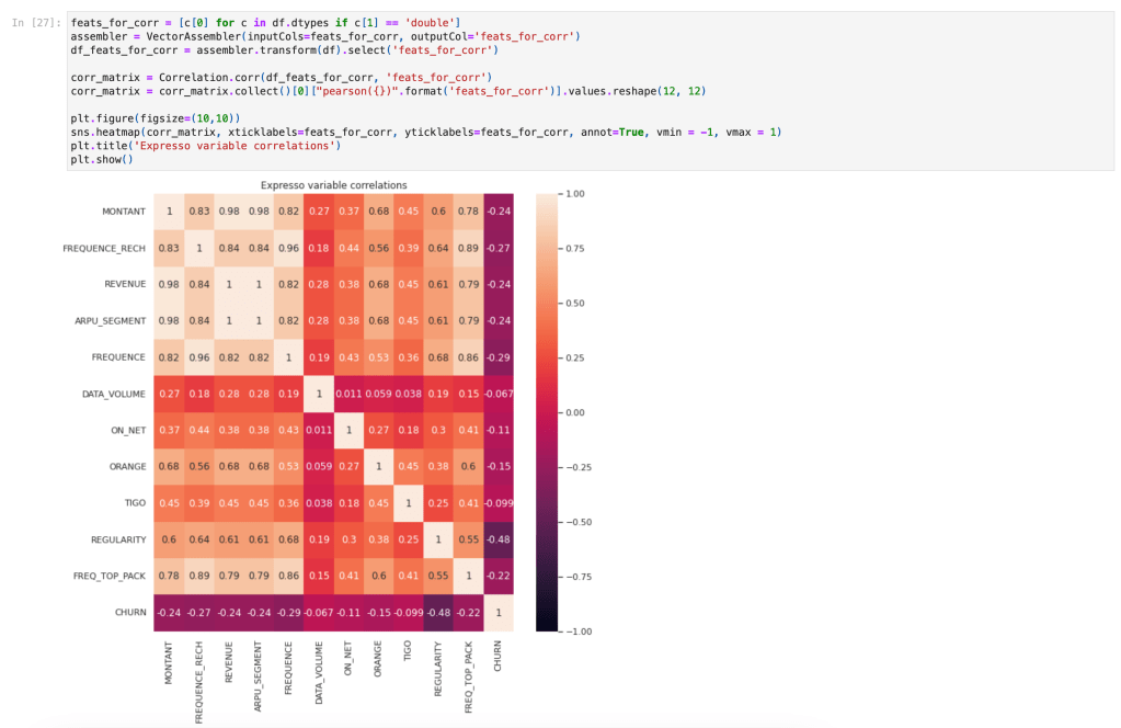
This was dramatically demonstrated for me during the EDA phase where I was attempting to produce a correlation matrix. It was a simple step that I needed in order to complete my EDA, but the operation simply would not complete no matter what I tried! After reading this tip, I did further research and came across the pyspark.ml.stat.Correlation function which gave me the result I wanted in just moments!

Building blocks

Resilient Distributed Datasets

RDD’s are the fundamental data structures of PySpark. Technically they are a “distributed collection of immutable Java Virtual Machine (JVM) objects” that can be processed in parallel. RDD’s are schemaless (meaning, unlike familiar tabular formats, they have no pre-defined data structure). A set of standard transformation methods are available for RDD’s which provide a lot of flexibility, for example map, filter, flatMap, sample, and so on. RDD transformations are “lazy” in that they only evaluate when an action is executed like take or collect. This lazy behaviour enhances performance as Spark can optimize complex data transformations at run time.

PySpark DataFrames

DataFrames are a higher-level abstraction on top of RDDs. They allow for working with structured data in the familiar tabular format, just like Pandas, and also provide a further speedup in performance. However, as Drabas & Lee point out you need to “temper your expectations” as there are many differences and limitations! Nonetheless a large number of methods are available for the DataFrame which are well-documented, and reading that documentation is necessary as the syntax and the underlying logic is often quite different to Pandas! For example here is a snippet showing how I obtained the % of nulls per column in my dataset:

	df.createOrReplaceTempView("sql_table")
	spark.sql(f'''SELECT
	TENURE
	, COUNT(*) AS totals
	FROM sql_table WHERE MONTANT > REVENUE
	GROUP BY 1 ORDER BY 1''').show()

view raw pyspark_sql.py hosted with ❤ by GitHub

Coming from a SQL background, I was delighted to find that data wrangling could also be performed using SQL-like syntax, which I used this quite extensively in the project. For example, here is a snippet showing how to use SQL syntax to get the number of customers by tenure where one variable is greater than another:

	df.agg(*[
	(fn.round(1 – (fn.count(c) / fn.count('*')), 4)).alias(c + '_%nulls')
	for c in df.columns
	]).show(vertical = True)

view raw pyspark_aggregation.py hosted with ❤ by GitHub

Built-in functions

You’ll notice in the first snippet above I made use of fn.round() and fn.count() – there is a long list of built-in Spark SQL functions, which will definitely come in handy when working in this space: everything from simple rounding to more complex functions like levenshtein distance are available.

Feature preparation

Working with features and preparing them for input into models was also different in PySpark, but again it is all well-documented. The trick is in figuring out how to proceed to get the desired outcome for your use case. One key difference is that PySpark models expect features as a vector of columns so the VectorAssembler is a crucial component. Being familiar with Scikit-Learn, using a Pipeline to handle feature preparation was, however, intuitive.

Modelling

I used the CrossValidator to experiment with three of the available classification / regression models and various parameter combinations within each to determine which would work best for this dataset. These were the results:

Model	Mean Runtime	areaUnderROC
LogisticRegression	10.9883 seconds	0.9264
RandomForestClassifier	47.7957 seconds	0.9289
GBTClassifier	74.7850 seconds	0.9309

From the above we can see that in terms of our metric, areaUnderROC, all three models produced results that were quite similar. However LogisticRegression was considerably faster. In business this is often a powerful deciding factor, both because of cost implications, and the requirement to train and predict on a fast turnaround if required. For this reason I used LogisticRegression as my final model of choice, even though (but only by a small margin) it had the lowest areaUnderROC.

The final areaUnderROC obtained on the hold-out test set using LogisticRegression was 0.9255 which was very similar to the metric obtained via cross-validation (0.9264).

Performance tricks

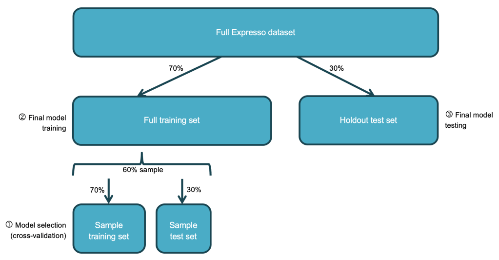
One of the biggest gains in performance I secured was by persisting the training set prior to cross-validation so that it could be read from memory during the many iterations of cross-validation instead of from disk. This reduced my cross-validation times by 29% on average. I also ran cross-validation on just a 60% sample of the training set, which further reduced runtimes without any significant impact on results:

I experimented with various other performance recommendations. For example, I read that cross-validation “parameter evaluation can be done in parallel by setting parallelism with a value of 2 or more (a value of 1 will be serial) before running model selection with CrossValidator”. I used the parameter (cautiously with a value of 2 since the same documentation warned about exceeding cluster resources!) and it resulted in modest performance gains. I had also read that using a larger number of smaller partitions could improve performance so I tried repartitioning my data into 4 partitions, but the runtimes were very similar so in the end I went with the default of 2 partitions.

Conclusions

If you’re already familiar with data and machine learning principles, then transitioning to the Apache PySpark environment is quite do-able. A deeper understanding of the underlying architecture is definitely useful, and paying close attention to how things are realised within this framework (as opposed to what you think you know from prior experience!) is definitely advisable. Once I got used to the environment I thoroughly enjoyed doing this project!