Natural language processing algorithms work with numbers, not text. So how can we convert strings of text into numbers that are representative of the meaning of that text? Some of the simplest methods (which can be surprisingly effective for some applications) are those that count words in various ways. In this article I’ll unpack the following 3 options:

• Bag-of-words (BOW)
• Term frequency (TF)
• Term frequency – Inverse Document Frequency (TF-IDF)

These methods all produce what is known as a term-document matrix. In this matrix columns represent all the words in the vocabulary of the corpus, and rows represent the words present in each document of the corpus.

ScikitLearn provides a very simple example – a tiny corpus of 4 strings – which can help us understand the mechanics of each method:

[‘This is the first document.’,
‘This document is the second document.’,
‘And this is the third one.’,
‘Is this the first document?’]

The Bag-of-words (BOW) approach simply asks whether each word occurs in the given document – the output is a binary value. For example we would represent the second document in our corpus as a vector like this:

and	document	first	is	one	second	the	third	this
0	1	0	1	0	1	1	0	1

To implement this option you can use ScikitLearn’s CountVectorizer with the parameter binary = True.

The Term frequency (TF) method instead asks how often each word occurs in the given document – so the output is an integer. The second document in our corpus would therefore be represented as follows (note 2 where the word ‘document’ appears twice):

and	document	first	is	one	second	the	third	this
0	2	0	1	0	1	1	0	1

To implement this option you can use ScikitLearn’s CountVectorizer with the parameter binary = False.

Jurafsky & Martin illustrate how this might be meaningful using just 4 words from 4 Shakespeare’s plays:

	As You Like It	Twelfth Night	Julius Caesar	Henry V
battle	1	0	7	13
good	114	80	62	89
fool	36	58	1	4
wit	20	15	2	3

We can immediately see that As You Like It and Twelfth Night, as comedies, contain plenty of references to fool and wit – where Julius Caesar and Henry V, as tragedies, contain many more references to battle. These 4-word vectors would allow us to gauge that the two comedies contain more similarities, and so also with the two tragedies.

Note that ‘terms’ may be individual words as in the example above OR n-grams, which can be a useful option to experiment with  in some contexts. For example with the parameter ngram_range = (2, 2) CountVectorizer will produce bigrams and their counts such as ‘This is’, and ‘is the’, etc.

The Term frequency Inverse-Document Frequency (TF-IDF) method refines on the simple counting techniques described above by introducing the IDF component – essentially a measure of the sparseness of terms in a corpus – using the following formula, where t denotes a term:

The idea behind the IDF concept is that the fewer documents that contain a term, the more likely it is that the term is important in those documents that do have it. Consider the word ‘is’ from our mini-corpus above. It occurs in every document so its IDF is calculated as follows:

Whereas the word ‘second’ only occurs in one document so its IDF is calculated as follows:

TF-IDF is the product of TF and IDF, so it is calculated as follows:

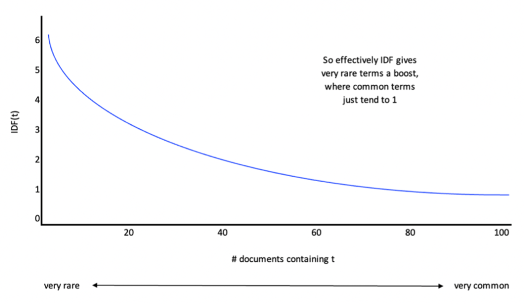
The following graph illustrates how effectively IDF gives rare terms a boost where with very common terms like ‘is’ the IDF tends towards 1 so these terms will hardly be boosted at all:

To implement this method you can use ScikitLearn’s TfidfVectorizer which produces a normalized TF-IDF output (note ScikitLearn adds 1 to the numerator and denominator of the IDF formula to avoid the possibility division by 0).

The second document in our corpus would therefore be represented as follows (the word ‘document’ which occurred twice is still the most important, but we can see that rare word ‘second’ has been slightly boosted by the IDF score where common words like ‘is’ and ‘the’ have lower scores):

and	document	first	is	one	second	the	third	this
0	0.6876	0	0.2811	0	0.5386	0.2811	0	0.2811

As you may imagine, all 3 of these methods produce sparse vectors: the average vocabulary in a corpus will be large, whereas the number of words used in each document will be quite limited. Some algorithms handle sparse vectors without issue – for example when using Naïve Bayes for sentiment analysis. In fact Jurafsky & Martin note that using the simplest BOW approach for this application can sometimes yield better results than TF or TF-IDF: “for sentiment classification and a number of other text classification tasks, whether a word occurs or not seems to matter more than its frequency”! However, many algorithms work best with dense vectors, so in the next article we’ll look at embeddings.