For this project I followed the universal workflow of machine learning as described in Deep Learning with Python (1^st edition) by François Chollet. It is a classic text which builds the student’s understanding of neural networks ‘brick by brick’ and was the first book that really gave me a good understanding of where to start with neural networks, and how to build on that start to realise incremental improvements in performance.

I completed the project on my local machine (an M1 MAC) as I was interested in testing its GPU capabilities. It proved quite doable, but also a little fraught. At the time South Africa was experiencing heavy load-shedding and the power would be unavailable for anything from 2-4 hours at a time (you do not want your machine to run out of battery after you’ve been training your neural network for 3 hours!). Furthermore it was summer and the MAC ran quite hot when using the GPU so I had a little USB fan connected trying to cool it off (which worked surprisingly well – but I also worried about it drawing more power!). All-in-all, however the job was done 👍.

Defining the problem and assembling a dataset

The project centred around using convolutional neural networks and transfer learning for the task of multi-class classification of images. As a keen bird-watcher, the Kaggle dataset BIRDS 475 SPECIES- IMAGE CLASSIFICATION (Piosenka, 2023) * piqued my interest. For humans, many birds are easy to identify, having distinctive colours or shapes, while others – famously known as LBJ’s or ‘Little Brown Jobs’ – can be quite tricky as they may be quite drab and lack easily distinguishable features.

* Unfortunately the dataset has subsequently been removed from the Kaggle platform.

The original dataset covered just 100 bird species. However, the dataset was updated just 2 days prior to my starting the project, and the version that I worked with (Version 61) contained images for 475 bird species. In this version we were told to expect ‘75,394 training images, 2375 test images (5 images per species) and 2375 validation images (5 images per species).’

Piosenka was rather informative about how the dataset had been compiled, including the following information relevant to decisions I faced on the project:

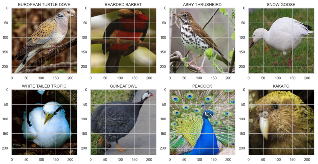
• This is a very high quality dataset where there is only one bird in each image and the bird typically takes up at least 50% of the pixels in the image.
• All images are 224 x 224 x 3 color images in jpg format.

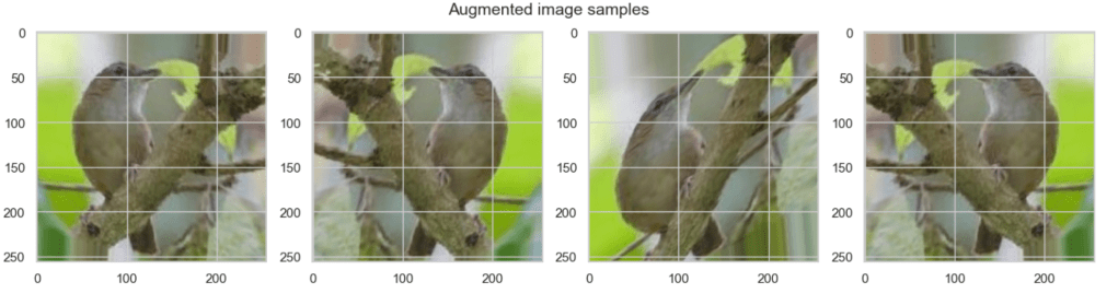
Below is a sample of how the images looked:

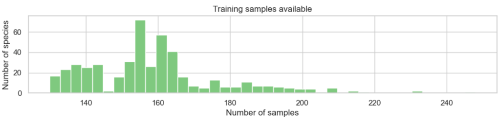
• The training set is not balanced, having a varying number of files per species.
• However each species has at least 130 training image files.

Here we can see that all species did indeed have at least 130 training images, but some had considerably more:

This comment was important:

• The test and validation images in the data set were hand selected to be the “best” images so your model will probably get the highest accuracy score using those data sets versus creating your own test and validation sets. However the latter case is more accurate in terms of model performance on unseen images.

And finally the following issue was noteworthy:

• One significant shortcoming in the data set is the ratio of male species images to female species images. About 80% of the images are of the male and 20% of the female. Males typical are far more diversely colored while the females of a species are typically bland. Consequently male and female images may look entirely different. Almost all test and validation images are taken from the male of the species. Consequently the classifier may not perform as well on female specie images.

As a bird-watcher, I am familiar with this issue: in practice one often waits for the male of a pair to make an appearance before being able to identify the species with certainty – so practically it skews the dataset towards how a human would go about (and also likely struggle with) identification.

Choosing a measure of success

While not every class was equally likely (given the slight imbalances in the number of samples we had per species) that imbalance was not very severe so I chose accuracy as my evaluation metric, since our main interest was in the percentage of images correctly classified:

Deciding on an evaluation protocol

As mentioned, the validation and test sets by default each contained 2375 images (5 images per species). For performance reasons, I was keen to avoid using kfold cross-validation, but at the same time I felt that the validation and test sets were a bit on the small side. In addition, Piosenka had mentioned that the validation and test sets contained the ‘best’ images which might lead to overly favourable results compared to real performance on unseen images of varying quality (and gender). For these reasons I took the decision to re-combine the given training / validation / test sets, and then do my own split. There were a total of 80144 images, which I split as follows:

• Train (70%)
• Valid (20%)
• Test (10%)

Because of the slight imbalance in the dataset I used stratified sampling to do the split. Having done so, I used a simple train / validation cycle to evaluate my results. And of course the test set was reserved for testing the final model selected based on the validation results.

Preparing your data

Re-working the train / validation / test split

The Keras ImageDataGenerator has a handy flow_from_dataframe method (Keras, 2023), so you can re-organize the data in a dataframe, without the need to actually move images into different directories to employ a different split. You simply need a dataframe with filepaths and labels. The csv supplied with the dataset already contained this information:

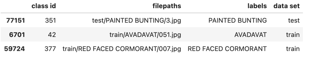
All that remained was to perform stratified sampling on it to re-organize it into the 70 / 20 / 10 ratios discussed above.

Setting up image data generators

There are a few considerations when it comes to setting up data generators for computer vision:

• Using a generator is essential: we would not want to attempt to load all 56088 training images into memory before training (certainly not on my laptop anyway!)
• Then as Chollet points out ‘data should be formatted into appropriately preprocessed floating-point tensors before being fed into the network’ (2018, p.135).
• We also need to feed the data to the network in batches. A smaller batch size will generally converge quicker, if slightly less accurately, so I went with a size of 64 here (Brownlee, 2019).
• And finally, it is very typical to make use of data augmentation techniques to prevent overfitting.

There are many data augmentation options. However, because our bird images were all rather nicely positioned within frame, I elected to implement just 3 simple techniques:

• rotation_range which will rotate the images randomly by up to 15 degrees in each case
• shear_range which will ‘lean’ the image over by up to 15 degrees in each case
• horizontal_flip which will give a mirror image of the bird

I built this in as an option, but started with the vanilla images for the baseline models – more on data augmentation later!

Developing a model that does better than a baseline

Because there are many successful pre-trained models available (for example VGG, ResNet, Inception, MobileNet, and so on), and because training state-of-the-art models from scratch can be expensive, I would normally use transfer learning as the starting point for any computer vision task. However, for this assignment I decided to first explore what I could achieve as a baseline by building a simple convolutional neural network from scratch (because I was a student and this is the kind of thing students make time to explore because it’s interesting!).

Basic architecture considerations

Convolutional neural networks stack up Conv2D layers and MaxPooling2D layers, the outputs of which are transformed into a format appropriate for feeding into a conventional network of one or more Dense layers which will deliver our final prediction. Because of their structure they efficiently condense key feature information, and are therefore faster to train than regular Dense networks. The model architecture influences not only the performance of the network but also the inherent viability of the size of the network (especially given limited hardware resources). The objective with my first network was to train a basic Convnet that achieves statistical power. Remember we saw earlier that the class with the most samples has 248 images out of a total of 80144 images in the dataset, so a common sense baseline would equate to ~248/80144 or ~0.003. Our model needs to do better than that! I considered the following aspects when designing this initial basic model:

Convolutional layers

The Conv2D layer is effectively a set of filters that are passed across each image, producing feature maps. Each feature map learns to detect a different image feature (like an edge, a colour, a texture, and so on). Below is a depiction of what is happening with only 1 colour channel. For RGB the same principles apply but the depth is 3 for the 3 colour channels.

• The kernel_size of the filter is typically either 3×3 (shown below) or 5×5.
• The number of filters determines the number of features learned. It is typical to increase the number of filters in each consecutive convolutional layer, e.g. 32, 64, 128, etc.
• The stride represents the number of pixels to move the filter at each iteration.
• The activation function gives us a non-linear output: relu is very typical.

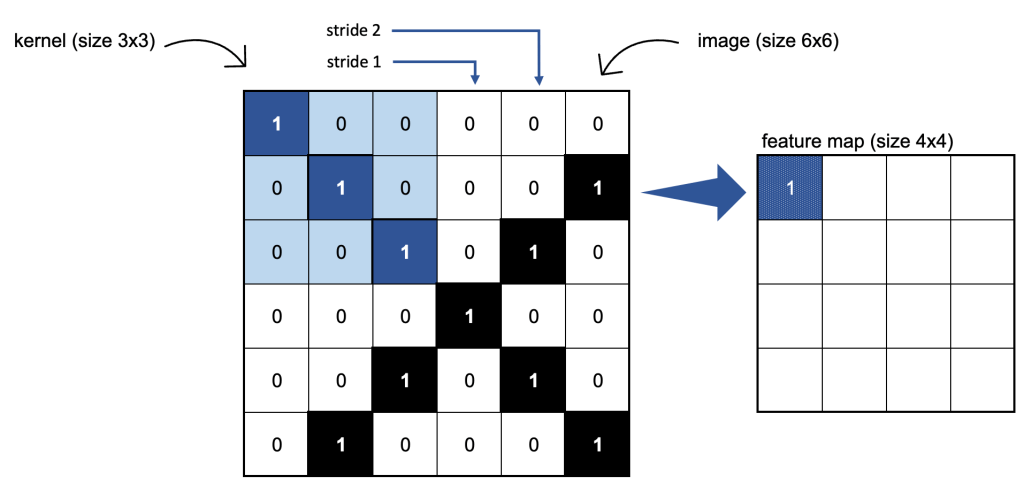
I opted to stack 3 Conv2D layers, where the number of filters increased from 32, 64, to 128. As Chollet notes adding layers ‘serves both to augment the capacity of the network and to further reduce the size of the feature maps so they aren’t overly large when you reach the Flatten layer’ (2018, p.133) – more on this in a moment. I chose a kernel size of (3, 3) and a stride of 1 in all but the first layer where I used a stride of 2. This latter decision was largely based on keeping the size of the network manageable.

Max pooling layers

The MaxPooling2D layer further condenses the information: we effectively apply another (non-overlapping) filter to the feature map by simply selecting the maximum value found within each filter space:

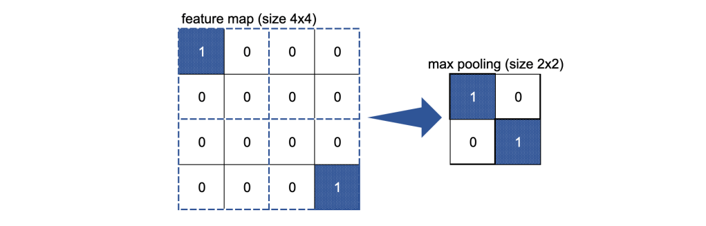
I have used a filter of size (2, 2) for each MaxPooling2D layer.

Global average pooling layer

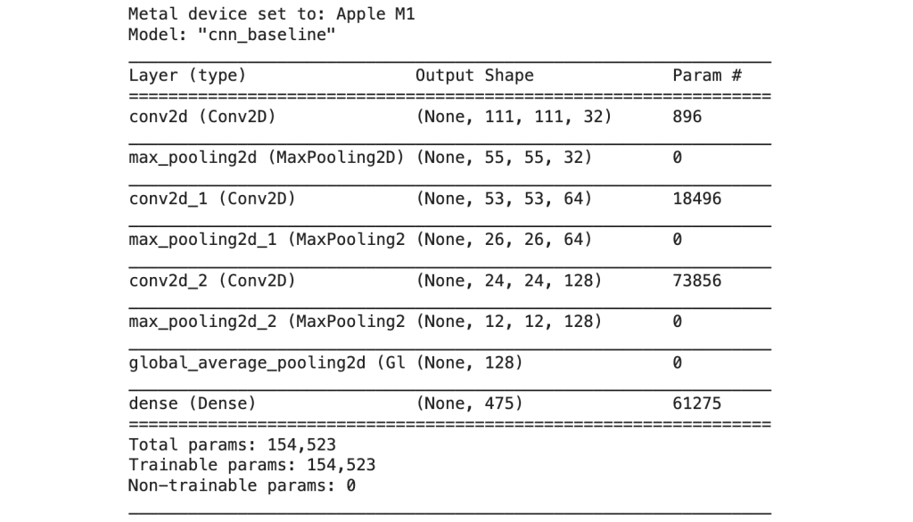
As our last step we want to feed the outputs of our stacks of Conv2D and MaxPooling layers into a conventional densely connected classifier network. The outputs from the convolutional part of our network are 3D tensors, however, the Dense layer expects inputs as 1D vectors. Chollet uses a Flatten layer which transforms the outputs of our convolutional network into a 1D format, ready for the next steps. However, I noticed that this resulted in an explosion in the number of trainable parameters so I decided to do a little further research, and came across a very illuminating article by David Landup (2022) suggesting that GlobalAveragePooling2D would be more effective. This is because instead of just transforming the shape, we are taking the average of each feature map from our convolutional network: ‘It applies average pooling on the spatial dimensions until each spatial dimension is one, and leaves other dimensions unchanged. For example, a tensor (samples, 10, 10, 32) would be output as (samples, 1, 1, 32)‘ (Anon., 2021). Initially, when using a Flatten layer my network had 3,073,179 trainable parameters. By using a GlobalAveragePooling2D layer instead I reduced the number of trainable parameters to just 154,523!

Dense layer

The size of my final Dense layer is determined by the number of classes: 475 classes. The softmax activation function is used for this final layer which is also our output layer. It is appropriate for multiclass classification because it will return 475 probability scores, where each score will be the probability that the current image belongs to one of our 475 bird species. These probabilities all sum to 1, and the species with the largest probability will be the predicted category.

Experiment 1 – very basic CNN baseline

And so finally I was ready to run my first experiment.

Model architecture

The initial model architecture had a total of 154,523 trainable parameters:

Compiling the model

Loss function

The categorical_crossentropy loss function is typically used for multi-class classification problems and I used throughout in all my experiments.

Optimizer and learning rate

I chose to use Adam as the optimizer: it is a popular choice, known for achieving good results fast by combining the benefits of AdaGrad and RMSProp (Brownlee, 2021). For this experiment, I left the learning rate at the default (0.001) as this iteration was all about investigating preliminary results.

Fitting the model

At this point we could fit our first model and evaluate the results. Note that when using a data generator the data is generated endlessly so model.fit() needs to know how many samples to draw for training (steps_per_epoch) and validation (validation_steps).

Our training data has 56088 images, and we’re using a batch size of 64. That gives us 56088/64 = 876 as our steps_per_epoch. Similarly our validation data has 15859 images, which gives us 15859/64 = 248 as our validation_steps.

I limited training to 20 epochs to get an initial feel for how the network performed.

ModelCheckpoint

It is useful to save the best model achieved as the epochs progress so that if, for example, we find the best model was achieved after only 3 epochs of training we don’t have to retrain the model to get those weights – we can simply load the weights of that best model and use it for prediction. I therefore implemented the ModelCheckpoint callback as a best practice.

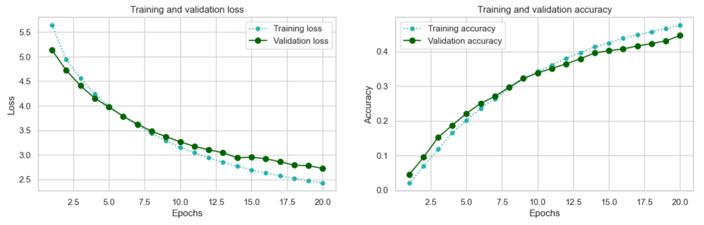
With this basic model, we certainly achieved statistical power, with ~0.45 accuracy being far superior to just guessing (remember our common sense baseline was ~0.003).

After 20 epochs validation loss is still decreasing and validation accuracy is still increasing. In addition validation and training loss, and validation and training accuracy are still tracking quite closely. We could continue to train for more epochs until we see signs of overfitting. However, at this point I am going to shift my focus to transfer learning, as this is the approach that generally makes the most sense for basic computer vision tasks such as this one: leverage a pre-trained network for faster, and usually superior results.

Scaling up: developing a model that overfits

Convnets trained on one set of tasks can readily be re-purposed for other tasks for 2 main reasons (Chollet, 2018, p.123):

• many of the patterns they learn are translation invariant , in other words if a pattern like a particular type of edge is learned, it can be recognised at any location in any picture
• they learn spatial hierarchies of patterns, so initial patterns learned will be generic to many images

It makes sense to ‘scale up’ by leveraging the power of one of these pre-trained networks. There are a number of open source pre-trained models available. I selected MobilenetV2 (Keras, 2023) because it was designed to operate with minimal resources on mobile devices, and it’s a relatively fast model at an estimated 3.8ms per inference step on GPU (Keras, 2023).

The authors of the original paper introduce the model as ‘significantly decreasing the number of operations and memory needed while retaining the same accuracy’ (Sandler, et al., 2019). They go on to explain ‘Our main contribution is a novel layer module: the inverted residual with linear bottleneck. This module takes as an input a low-dimensional compressed representation which is first expanded to high dimension and filtered with a lightweight depthwise convolution. Features are subsequently projected back to a low-dimensional representation with a linear convolution.’

As with all pre-trained networks, there is a final section (in this case a GlobalAveragePooling layer followed by a Dense layer) which we can replace with our own Dense classifier which will learn the specific task of distinguishing between our 475 bird species. This approach is known as feature extraction.

Experiment 2 – feature extraction

Each pre-trained model expects input data to be in a specific format and MobilenetV2 is no exception. The Keras documentation advises ‘For MobileNetV2, call tf.keras.applications.mobilenet_v2.preprocess_input on your inputs before passing them to the model. mobilenet_v2.preprocess_input will scale input pixels between -1 and 1.’ (Keras, 2023).

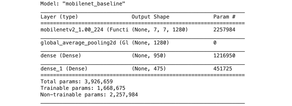
My initial architecture consisted of the pretrained MobileNetV2 network as the base, excluding that final Dense portion of the network I mentioned (parameter include_top = False). Because we do not want to re-train the MobileNetV2 weights we make sure that the trainable parameter is set to False so that the original weights will be preserved during the training process.

I then added my own Dense network on top of this base: a GlobalAveragePooling2D layer (which efficiently transforms the data into a 1D tensor ready for input), followed by an intermediate Dense layer with 950 neurons using relu as the activation function and a final Dense output layer with 475 neurons using softmax as the activation function which, as explained above will return a set of 475 probabilities, one for each bird class. The original MobileNetV2 network only had one Dense layer, but I decided to go with two for extra capacity in light of the large number of classes my dataset has (many of which are quite similar to one another). I’ll compare these results with a smaller network later.

The new model was a network with 1,668,675 trainable parameters:

In compiling the model I went with exactly the same settings as before: categorical cossentropy for the loss function and Adam for the optimizer. The default learning rate of 0.001 again made most sense as a ‘first pass’ to get a feel for how the network peforms. Because of using a pre-trained network as a base I expected the performance to increase more quickly than the ‘from scatch’ CNN baseline model of experiment 1 so I opted to train for an initial 15 epochs in order to assess the results:

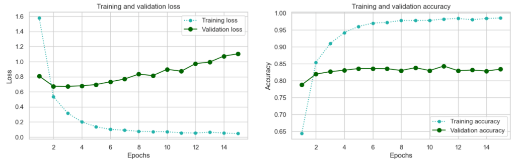
The increase in accuracy to 0.84 is an immediate vindication for the transfer learning approach! Using TensorBoard to compare the loss and accuracy metrics for experiment 1 with those of experiment 2 – there is a stark difference:

However, we are seeing overfitting from epoch 4 when the validation loss starts to increase – if we can combat this, improvements can be reaslised.

Regularizing your model and tuning your hyperparameters

To combat overfitting and promote convergence I tested incorporating 4 measures:

• data augmentation
• batch normalization
• dropout
• a lower learning rate

Fitting the model to augmented data

Chollet describes the benefits of data augmentation as follows: ‘Data augmentation takes the approach of generating more training data from existing training samples, by augmenting the samples via a number of random transformations that yield believable-looking images. The goal is that at training time, your model will never see the exact same picture twice. This helps expose the model to more aspects of the data and generalize better.’ (2018, p.139)

What I found important to understand was how this really works. The term ‘augmentation’ almost sounds like you might be able to use it to generate additional images per epoch for training. This is not the case: rather it varies the images each time they are passed to the model. Let’s say we have just 100 images for training. During training we will pass 100 images to the model to train on within each epoch – but instead of passing exactly the same 100 images each epoch, we’ll pass variations of those images: so the images that you train on in epoch 1 will differ slightly (according to your data augmentation specifications) from the images you train on in epoch 2 and so on. In this way we avoid the model seeing exactly the same image each epoch, which helps it to generalize better.

Such augmentation measures are only performed on the training set of course: the validation and test images remain as-is.

Batch normalization

Chollet tells us in the second edition that ‘Although the original paper stated that batch normalization operates by “reducing internal covariate shift,” no one really knows for sure why batch normalization helps.’ Nonetheless, he adds: ‘In practice, the main effect of batch normalization appears to be that it helps with gradient propagation’ (2021, p.256)

His strong recommendation is to place batch normalization after a Conv2D or Dense layer, but before activation and I have followed this recommendation below.

Dropout layer

Dropout ‘consists of randomly dropping out (setting to zero) a number of output features of the layer during training’ and ‘the dropout rate is the fraction of the features that are zeroed out; it’s usually set between 0.2 and 0.5’ (Chollet, 2018, p. 109). I’ll be adding a dropout layer of 0.4 to mitigate against overfitting.

Experiment 3 – feature extraction with overfitting measures

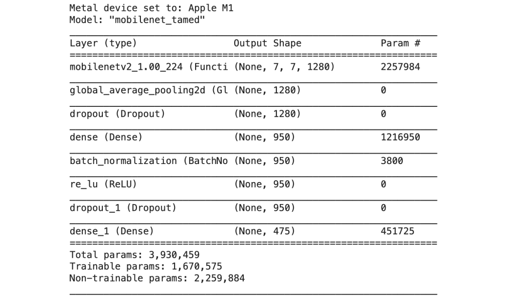
Here is the architecture for my ‘tamed’ version of feature extraction. There were a total of 1,670,575 trainable parameters:

Other adjustments

I reduced the learning rate from the default of 0.001 to 0.0005, so that our model would take smaller, more conservative steps towards a good local minimum, or hopefully even a global minimum. In compensation for the lower learning rate I also increased the number of epochs to 20.

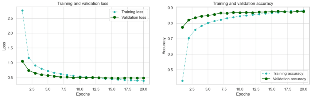
This is a substantial improvement. Performance reaches its peak after sixteen epochs but we have gained an improvement of over 3 percent on our original mobilenet_baseline model at 0.8776!

You may wonder at the validation accuracy being more-or-less consistently higher than the training accuracy, and similarly the validation loss being lower than the training loss: this is a common phenomenon seen when using Dropout during training – the network capacity is limited at training time as a result of dropout, but the full capacity is used during validation.

This is rather a decent result, but can we do better by using a simpler architecture – as the developers of MobilenetV2 did?

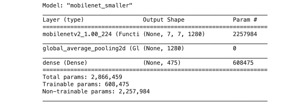
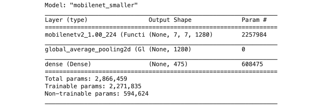
Experiment 4 – feature extraction with a smaller network

The original top layer of MobileNetV2 consists only of a GlobalAveragePooling2D layer followed by a Dense layer which produces the final predictions. I was interested to compare the results of this smaller Dense network architecutre with my larger architecture from experiment 3. In this iteration, I continued to make use of data augmentation which is really a ‘best practice’ in image recognition tasks, and I also retained the lower learning rate of 0.0005 as I wanted to guard against the model converging too fast on a potentially sub-optimal minimum. As before I settled on training for 20 epochs in order to evaluate the progress of the model.

This model version had a total of 608,475 trainable parameters:

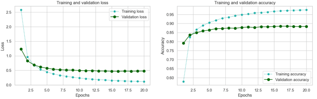
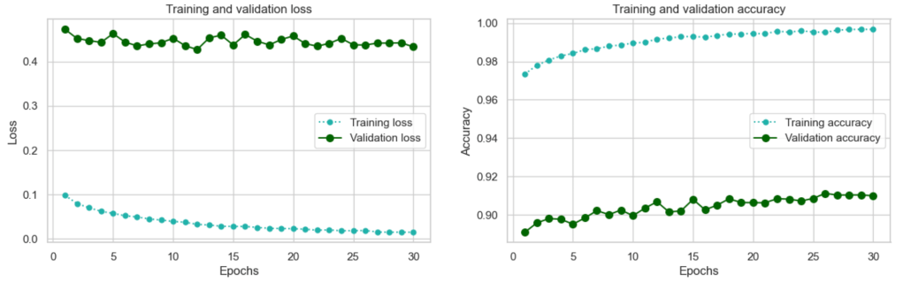
After 20 epochs this is how it was looking:

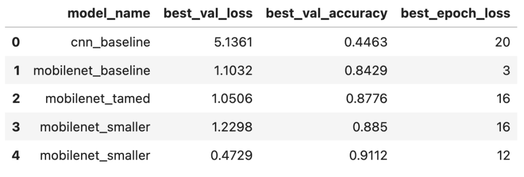
And here is an overview of the results for all 4 models:

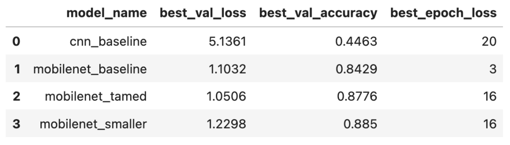
From the above it would appear that in fact the smaller model of experiment 4 performed slightly better than the larger ‘tamed’ model of experiment 3. A gain of >~0.01 accuracy is still significant in machine-learning terms although it sounds small! However, we are seeing signs of overfitting after epoch 16 where the validation loss seems to plateau.

Fine-tuning

Now that we are seeing reasonable results from feature extraction we can go to the next level which is fine tuning. ‘Fine-tuning consists of unfreezing a few of the top layers of a frozen model base used for feature extraction, and jointly training both the newly added part of the model (in this case, the fully connected classifier) and these top layers.’ (Chollet, 2021, p. 234). You fine tune a classifier that has already been trained to your specific task – as we did in experiment 3 and 4 above – otherwise ‘the error signal propagating through the network during training will be too large, and the representations previously learned by the layers being fine-tuned will be destroyed.’ He further recommends that in this process we should not unfreeze any batch normalization layers. (Chollet, 2021, p.234)

Because experiment 4 achieved better results than experiment 3, I’ll be using the MobileNetV2 base with the smaller single layer dense network on top as a basis for fine-tuning.

Experiment 5 – finetuning

To proceed with finetuning the first step was to load the weights from epoch 16 of experiment 4 (which was my best epoch) and proceed from there.

There are 16 main blocks in MobileNetV2 and I applied fine-tuning from block 13. The process involved first setting the whole network to trainable, then refreezing the layers we did not want to train. The final model was trainable from block 13 onwards, excluding the batch normalization layers.

This resulted in a network with a total of 2,271,835 trainable parameters:

It is recommended to use a very low learning rate when fine tuning. Chollet explains: ‘The reason for using a low learning rate is that we want to limit the magnitude of the modifications we make to the representations of the three layers we’re fine-tuning.’ (2021, p.236). If the learning rate was too large we would reduce the quality of the feature representations learned in the original model. Here I reduce the learning rate to 0.00001.

Here are the results:

And here is an overview of the results for all 5 models:

Fine-tuning worked well: we again increased our validation accuracy by over 3 percent. In fact based on the trends (validation loss is still going down overall, and validation accuracy is still increasing overall) it would be worthwhile training for more epochs – there is potential there for improvement. However, in the interests of time I am now going to turn to training our final model and evaluating it on the holdout test set.

Train the final production model and test

For the final test, I completed a training run on the full training set (training 70% + validation 20%): this constituted 16 epochs of feature extraction followed by 12 epochs of fine-tuning which represented our best results above. I then evaluated the results on the holdout test set (10%). The result was a test accuracy of 0.9095 compared with our best validation accuracy of 0.9112.

Looking at a summary of species accuracies, there were 294 species where an accuracy of > 0.9 was obtained:

With so many species a confusion matrix is not visually feasible! However, plotting the 20 worst classes was interesting:

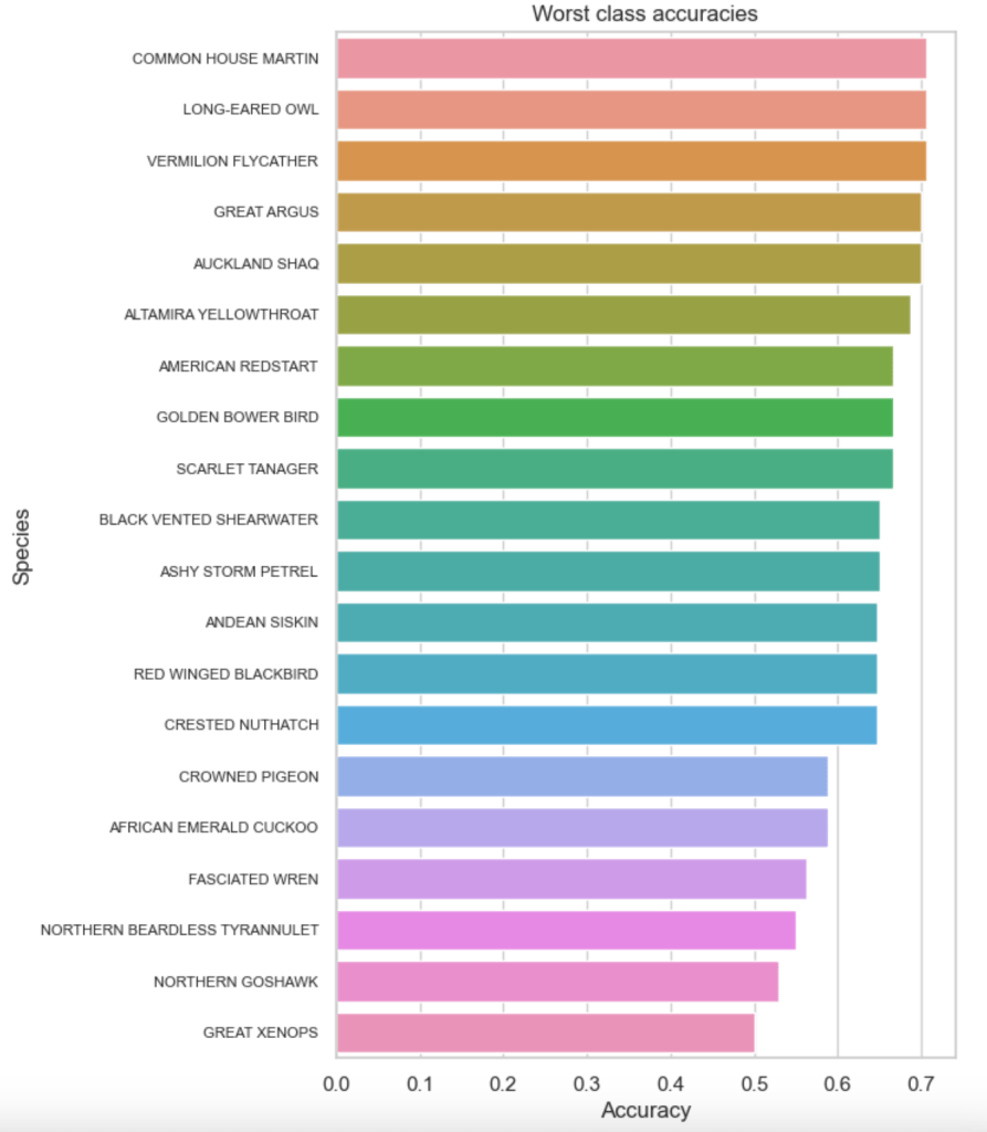
The worst performer was the GREAT XENOPS:

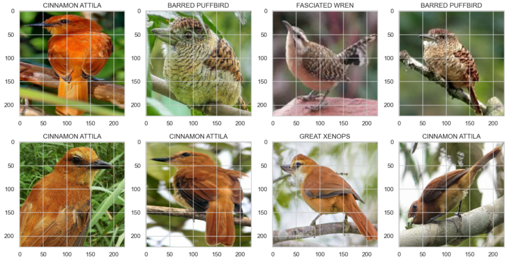
The similarities in colouring and form between the GREAT XENOPS and the CINAMMON ATTILLA are quite apparent. However the BARRED PUFFBIRDs obtained in the random selection above did not look particularly similar. But examining specific bird images I could find variants where that same distinctive rust colouring occurs which seems to be the possible source of confusion:

It’s a Panamanian bird that I am unfamiliar with, however such variations are common not only between males and females, but also between adults and juveniles. This is one of the aspects that makes bird-watching tricky for humans too.

The bird at the top of the list of ‘confused birds’ is the COMMON HOUSE MARTIN. This is a bird that I am familiar with and the confusion therefore did not surprise me. Let’s look at this bird and some of the species it was confused with:

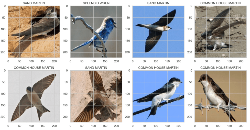
The sand martin is particularly similar-looking and as an amateur bird-watcher I can understand how the model would be confused!

A final test accuracy of 0.9095 was reasonable. If time had permitted one could keep tinkering of course! For example in experiment 5 we had not established if we had reached the boundary of the best performance we could obtain with fine-tuning, and given the low learning rate it is quite possible performance could continue to improve steadily for more epochs. I, however, had an assignment deadline so I had to call it quits at this point!

The full code for this project is available from my Github repo: