A/B testing is a popular technique for comparing two versions of a feature (A and B) to assess which will be most successful. It is widely used in the tech industry to provide a quantitative basis for decision-making, for example:
- Which web page style results in better click-through rates?
- Which recommender model results in improved user engagement?
- Which in-app message results in increased subscriptions?
- And many more!
This article will consider the following hypothetical scenario:
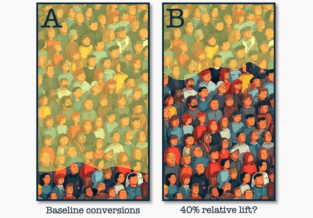
Your stakeholder wants to test a new version of an ad which they believe should result in more conversions. Their requirement for making it worthwhile is to see a 40% relative lift (or better) compared to the old ad.
The null hypothesis in A/B testing assumes there is no difference between the two ads. The hoped for outcome would be to reject the null hypothesis and find that there is a statistically significant difference between the two ads – in favour of the new version. Moreover this difference would need to be practically significant – in other words large enough to make a difference to the organization in context. Bear in mind that it may also be quite possible to find that the new version performs worse than the old one.
Interestingly, beyond tech, A/B testing can be used in other contexts where small iterative improvements can have a large cumulative effect over time – for example this article from Stanford Social Innovation Review describes a powerful implementation of ‘rigrorous, rapid, regular’ A/B testing in the educational sector.
The planning stage of any A/B test is the most crucial step to ensure that decisions can be made confidently based on the results obtained. The following guide outlines the basics, as well as some more nuanced aspects that may be important to your stakeholders’ decision making processes.
Power analysis
Power analysis is the foundational step of any A/B test, ensuring that your test will have enough statistical power to detect the effect you want to detect while guarding against over-optimistic conclusions. The four key variables of power analysis are:
- Minimum detectable effect
- Significance level
- Statistical power
- Sample size
In many scenarios you will decide upon (or know) what you want three of these variables to be, and will solve for the fourth one. The Python library statsmodels includes a function zt_ind_solve_power to do just this where your samples sizes are large enough (> 30). Let’s look at each variable in detail before diving into some hypothetical scenarios:
Minimum detectable effect
The minimum detectable effect (MDE) is often the starting point for your experiment, just as it is in our scenario. It asks the question:
“What is the minimum improvement that I need to see for it to be worthwhile implementing this change?“
For example here our marketing manager might say “I’m thinking of making a change to our subscription ad, but for it to be worthwhile I’d need to see at least a 40% improvement in conversions.” This could be termed relative lift. The MDE required is usually tightly coupled to the expected return on investment.
Now zt_ind_solve_power expects its parameter effect_size to be expressed as either Cohen’s d for continuous data (e.g the difference in effect size between 2 means) or Cohen’s h for binary data (the difference in effect size between 2 proportions).
The formula for Cohen’s d is as follows, where x̄ represents the mean of each group and spooled represents the estimated standard deviation of the combined groups (which could be estimated based on either historical data or domain knowledge):

The formula for Cohen’s h is as simpler calculation, where p represents the proportion of each group with a positive outcome:

In the case of the latter (which I’ll use in the rest of the examples) there is a very handy proportion_effectsize function in statsmodels, which we can make use of. So, for example, if our conversion rate is 0.05 and our stakeholder requires at least a relative lift of 40% this would equate to a new conversion rate of 0.07 or better. Using proportion_effectsize we see that this would translate into an effect_size, in Cohen’s h terms, of 0.084:
Significance level
The significance level, also know as α (alpha) asks:
“What’s the maximum chance I’m willing to accept of saying there is an effect when there really isn’t?“
We can view it as protection against obtaining a false positive. A significance level of 5% is very standard in both industry and academia, so if your stakeholder doesn’t specify, and the situation doesn’t suggest a specific requirement, then it is a good default option.
It is worth noting, however, that certain situations may call for an even more conservative (i.e. lower) significance level. For example, if you are testing a change to your payment gateway, a false positive might result in changing your user interface in a way that actually decreases the number of purchases made – resulting in financial losses. In this case you might choose an α of 1% so that stakeholders can have high levels of confidence in the test results before making a final decision.
Statistical power
Statistical power asks:
“If there really IS an effect of size x, what’s the chance I’ll detect it?“
We can view it as protection against obtaining a false negative. Setting the statistical power at 80% is very standard in both industry and academia and is a good default option.
However, in some situations it may be worth either increasing or decreasing the statistical power. A higher statistical power, say 90%, might be called for if the cost of losing a potential market opportunity due to a false negative would be high. Similarly a lower statistical power, say 70%, might be warranted if you want to run quick low-cost experiments to get a feel for preliminary results in order to establish whether it’s worth investigating further.
Sample size
This is often the variable that is being solved for in power analysis! You have defined the 3 objectives as outlined above and the question now is:
“How many samples do I need to include in my experiment to meet these objectives?“
What is worth considering here is not only the total sample size required but also over what period of time you expect to gather that data. For example, if you need a total sample size of 50,000 users but you only get 5,000 users to your site each day then it will take you a minimum of 10 days to collect sufficient data to analyze the results. There may also be instances where, due to say risk factors or expense, you only want to show a maximum of 1,000 users per day the changed feature – in this case it will take even longer to collect sufficient data to draw your conclusions.
In addition, as we will see, the ratio between treatment group size and control size is an important consideration. Let’s look at some scenarios to understand how each factor may influence the others.
Investigating options
Changing sample size ratios
If we assume that our MDE is 40%, as described above, or Cohen’s h = 0.084 and that we have chosen to stick with the industry standard statistical power of 0.8 and statistical significance of 0.05 – let’s now have a look at the effect of electing to use equal sample sizes, or not. The following code snippet shows how to solve for the control and treatment group sizes, given a changing ratio of control to treatment group:
Running this code for the following ratios, we can see that the more imbalanced the control and treatment sizes are the more uncertainty there is, and hence the more samples are required. When the control and treatment groups will be the same size (i.e. ratio = 1) the smallest number of samples is required:
| Ratio | Control size | Treatment size | Total samples |
| 0.25 | 5496 | 1374 | 6870 |
| 0.5 | 3297 | 1648 | 4946 |
| 1 | 2198 | 2198 | 4396 |
| 2 | 1648 | 3297 | 4946 |
| 4 | 1374 | 5496 | 6870 |
Changing power & alpha
Let us assume that we want to be conservative about how many people we show the new feature to, so we opt for a ratio = 0.25 so 1 treatment sample for every 4 control samples. We can now look at the effect of adjusting statistical power and alpha (using the same zt_ind_solve_power function shown in the snippet above):
| Power / Alpha | Control size | Treatment size | Total samples |
| 0.9 / 0.01 | 10419 | 2604 | 13024 |
| 0.8 / 0.01 | 8178 | 2044 | 10222 |
| 0.9 / 0.05 | 7357 | 1839 | 9197 |
| 0.8 / 0.05 | 5496 | 1374 | 6870 |
| 0.7 / 0.05 | 4321 | 1080 | 5402 |
It is immediately apparent the kind of tradeoffs that might need to be considered. If rapid, and potentially less expensive results are required the Power / Alpha combination of 0.7 / 0.05 might be the best option as we only need to collect a small number of samples (5402). But we are then sacrificing some statistical power so we’ll get a result quickly but there is a greater chance that we might miss a real effect that exists. On the other end of the scale if we are conservative about both Power and Alpha using the 0.9 / 0.01 combination we can place greater trust in the results but we need to collect a lot more samples (13024).
Beyond power analysis
Let us now say that we have settled on a ratio = 0.25 and we’ve agreed to go with the standard Power / Alpha combination of 0.8 / 0.05. We collect the indicated 6870 samples. And let’s also say that we see the desired relative lift of 40% when comparing the proportion of conversions in the control vs treatment groups. How much faith can we have in this result?
Statistical significance
The most basic question to ask is:
“Is my result statistically significant?“
To evaluate our test results we can use the statsmodels function proportions_ztest. The following code snippet shows how this would be done with the data we have assumed thus far:
The difference is statistically significant, yes: the chance that we would see a relative lift of this magnitude by chance is very small. But we also need to ask:
“Is my result practically significant?“
In this case it is practically significant because 40% meets the criterion set by our stakeholder. In other situations where you perhaps do not have such a clear mandate on what constitutes practical significance you will likely have to consider additional factors like potential return on investment and so on. BUT we also need to go one step further…
How confident can we really be?
The next question to ask is:
“What would be the confidence interval associated with a relative lift of 40%?“
Let’s see how we would determine this using the statsmodels function confint_proportions_2indep:
What this confidence interval is telling us is that if we were to implement this change in production it is 95% likely that the actual effect observed would be a relative lift of somewhere between 12.6% and 71.4%. If it were 71.4% you would be the hero of your department, but if it was only 12.6% it is likely your stakeholder would have sharp words for you! So what we are seeing here is that statistical significance does not equate to practical certainty. In some cases a higher threshold of certainty may be required before making a decision. Balancing the size of the treatment and control groups may help to an extent, but if our 1:4 ratio needs to remain in place we can also iterate over different sample sizes to determine an acceptable confidence interval – since the more samples we take, the narrower the confidence interval becomes.
Let us assume then that the stakeholder specifies the desired relative lift is 40%, but the lower bound of the confidence intervals needs to be at a minimum 30% in order to make a call on whether to proceed. We can use function confint_proportions_2indep to iterate through a range of sample sizes until we hit the desired minimum confidence interval of >30%. The following snippet demonstrates how this might work in practice:
The outcome really does illustrate the tradeoffs between the sample sizes you can afford to collect (and the time it will take to collect them) and relative uncertainty. If we were prepared to accept a higher degree of uncertainty we would only have to collect 6870 samples, but if we wanted to be very certain we’d need to collect 56870 samples!
In practice, these are decisions that would need to be made together with your stakeholders. What is important is to be able to give them a range of options, and also be able to clearly explain what the pros and cons of each are so that the appropriate approach is agreed on together.
Randomization is fundamental
It’s beyond the scope of this article but once you’ve decided on appropriate control and treatment sample sizes it’s essential that whatever method you choose to assign each sample to a group is random.
The above article explains: “Methods for achieving randomized sampling span two extremes. On one end, simple randomization requires minimal intervention, essentially encouraging you to do nothing. On the other end, more structured approaches ensure that both groups are carefully balanced to share similar characteristics.“
As always the approach you settle on will depend on the situation you are dealing with and the outcomes you need to achieve. There is no one-size-fits-all solution in this domain!
What if I have historical data?
In some cases data may have been previously been gathered and you’ll be asked to conduct A/B testing retrospectively. In this case, of course, you don’t have the luxury of structuring your experiment upfront: you have to work with what you have. What is important in this situation is to understand the provenance, potential, and limitations of the data at hand.
Let’s look at a sample dataset: Marketing A/B Testing (from Kaggle). The purpose of the dataset is to assess the effectiveness of an ad. “The majority of the people will be exposed to ads (the experimental group). And a small portion of people (the control group) would instead see a Public Service Announcement (PSA) (or nothing) in the exact size and place the ad would normally be.” Success or otherwise is indicated by whether they converted or not. In a real-life situation it would be particularly important to confirm whether the users in each group truly were randomly selected. If, for example, users visiting the site during the night were shown the PSA and users visiting the site during the day were shown the ad this would be non-random and the dataset would essentially unusable for the purpose of A/B testing. Being a test dataset we will proceed on the assumption that the random sampling methodology was sound.
It turns out there are a large number of samples and the dataset is extremely imbalanced – the ratio of ad to psa users is 24 to 1!
| test group | converted | count |
| ad | False | 550154 |
| True | 14423 | |
| psa | False | 23104 |
| True | 420 |
From these figures we can conclude that the conversion rates for each group are as follows:
Control group (saw no ads):

Treatment group (saw ads):

We can therefore also calculate the actual relative lift as follows:

Using statsmodel’s proportion_effectsize we can obtain the equivalent Cohen’s h of that relative lift which is 0.0530. Now the question that arises is this: if we assume we are aiming for the standard Power / Alpha combination of 0.8 / 0.05, and given the actual sizes of the treatment and control groups – what is the minimum detectable effect? The function zt_ind_solve_power can help us again, but this time we are solving for effect_size (where nobs1 = total sample size of the control group, aka ‘number of observations in sample 1’):
So we now know that with the respective sample sizes we have, we can detect an effect size of Cohen’s h = 0.0186, which is smaller than that actually seen in our data: Cohen’s h = 0.0530. Just for comfort though, Github Copilot provided me with the following function to convert from Cohen’s h back to relative lift, confirming that we could detect a relative lift as small as 14.26%:
Following the same method as before we can use the proportions_ztest to establish basic statistical significance (it is indeed significant with a Z-statistic of 7.4110 and a p-value: 0.0000000000!). We can then use confint_proportions_2indep to establish a confidence interval for that relative lift of 43% which turns out to be [33.6%, 53.1%].
Final words
It was tempting to title this article “How the pursuit of knowledge can be a bottomless pit” or “Down the rabbit hole with A/B testing” 🙃. The bottom line is that how you plan for and conduct each test will be very scenario-specific. It is therefore important to gather as much domain knowledge as possible, consider all stakeholder requirements and caveats, investigate which options could be feasible, and finally to present stakeholders with the main viable choices – clearly explaining their pros and cons. Ultimately they will usually be the ones making the decisions on how to proceed based on the outcomes of the A/B test you conduct.
