Before we dive into the theorems let’s tackle a concept one often sees in statistics: the notion of independent, identically distributed (iid) random variables. Whether we’re drawing a sample from a population or conducting a series of experiments like coin flips, we can assess whether iid holds true or not as follows:

Independent?

Here we are asking whether the value of one variable affects another.

Independence holds true for scenarios like these:

• Rolling a dice multiple times – the result of one roll does not affect the result of the next roll
• Measuring the heights of randomly selected people – the height of one person does not affect the height of another person (with the proviso that there may be exceptions like if two people are related, for example!)

Independence does not hold true for scenarios like these:

• Drawing cards from a deck without replacement – the result of the first draw (when 52 cards were available) will affect the subsequent draw (as there will now only be 51 cards available)
• Time series scenarios like looking at stock prices where the previous stock price has a bearing on the current stock price

Identically distributed?

Here we are asking whether all variables come from the same probability distribution.

Identical distribution holds true for scenarios like these:

• Flipping a coin repeatedly: there is the same probability of getting heads or tails each time, i.e. 50%
• Counting the number of articles users read each day on a website

This latter example took a bit of wrapping my head around. Instead of a normal distribution, looking at number of articles read per user will usually result in a long-tailed distribution rather like this one:

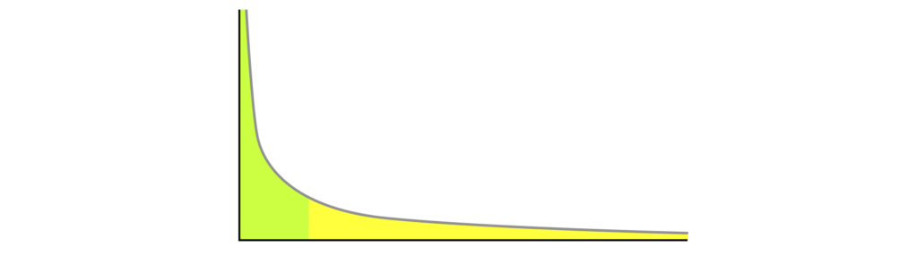
Long-tailed distributions are quite common in ‘real-world’ data! However, if we sample from this distribution, the variables are still coming from the same probability distribution, even though it’s not a normal one.

Identical distribution would not hold true if:

• Instead for sampling random users reading articles we sampled from 2 distinct groups like super-users and occasional users
• Similarly for the coin flips identical distribution would not hold true if we were to use 2 coins: one fair and the other loaded

So now we have this foundational concept out the way let’s look at two of the central theorems…

Law of large numbers

“The LLN states that given a sample of independent and identically distributed values, the sample mean converges to the true mean” (Wikipedia). In other words the more samples you draw from a population, or the more times you repeat an experiment, the closer the average result will be to the expected value. This is one of the key factors that makes statistical inference viable. We cannot measure the average height of all women in South Africa, but given a large enough sample where iid holds true we can reliably estimate what is true of the population mean based on the data from our sample.

Incidentally, LLN is also what makes casinos commercially viable: casinos may lose money on individual bets, but over a large number of bets the casino’s earnings will tend to be quite stable.

Central limit theorem

While LLN focuses on convergence to the mean, the CLT describes the distribution of the sample mean.

The CLT states that, provided enough samples are taken, the sample distribution of the sample mean will be normally distributed, regardless of the population distribution. And the more samples you draw, the more this will be the case.

So even if the population distribution is a long-tailed one like the one shown above, if we take enough samples (and this seems to be a surprisingly small number with 30 being the traditional minimum!), the distribution of the sample mean will tend towards a normal distribution like the one shown below:

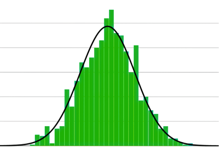
And the more samples we take, the more normality we will see. Gonzalez et al. note that “Many parametric hypothesis tests (such as t-tests and z-tests) rely on the assumption of normality to make valid inferences. These tests assume that the population from which the sample is drawn follows a normal distribution. The CLT comes into play by allowing us to approximate the distribution of the test statistic to a normal distribution, even when the population distribution is not strictly normal. This approximation enables us to perform these tests and make reliable conclusions.”

So even in the example mentioned above, where the number of articles users read each day on a website is a long-tailed distribution, if we were performing A/B testing we could use a t-test to determine whether the mean number of articles read by users on 2 versions of the site differed significantly or not.

If we are experimenting with ML models the CLT can be very helpful in determining a confidence interval for the mean accuracy across a series of experiments, provided sufficient experiments are run. I asked Deepseek-R1 for some more examples and this was an interesting one:

Moral of the story, LLN and CLT will frequently be mentioned in the context of statistics as well as machine learning so best to carry around in your own working memory what they mean at a high level as many applications are enabled by these foundations!