T testing – a worked example

A simple one-sample T-test

This variant on hypothesis testing is used when you have limitations, specifically:

The population standard deviation (σ) is unknown and your sample size (n) is <30

The fundamentals

The formula is a variant of what we’ve seen thus far, where x̄ = your sample mean, μ = a hypothesized population mean, s = the standard deviation of your sample, and v = n – 1:

Instead of a z-table, we’re going to use a t-table, where v = the “degrees of freedom” referenced for the final assessment.

Example

There is a theory that one should drink 2 litres of water each day. You’re wondering if Capetonians are managing this or drinking less on average each day. You survey 10 random Capetonians about their water drinking habits and get the following responses:

2.2, 1.2, 1.5, 1.8, 2.0, 1.3, 1.5, 1.7, 1.6, 1.5

It seems like most people don’t drink as much as 2 litres per day, but can you say the same for the majority of Capetonians?

Working it out…

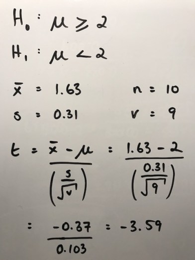
How does -3.59 compare with the “rejection region” score from our t-table? Well, assuming we’re after a 95% confidence level, if we go with the 9 degrees of freedom we have in this example, then for anything below -1.833 we can reject the null hypothesis:

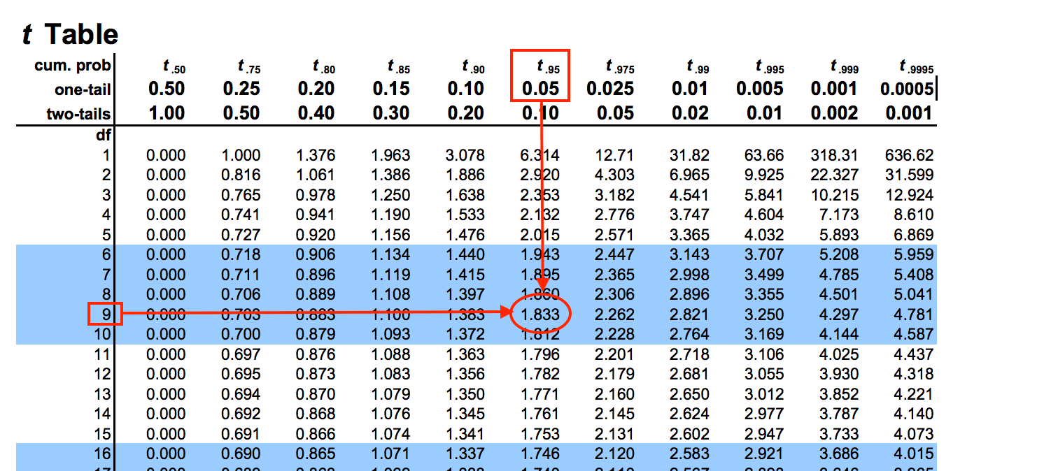
So it would seem that most Capetonians do not drink as much as 2 litres of water per day.

The stuff of imagination…

I put together this example to illustrate the principles, how the calculations work, and how the t-table works. In principle you can imagine how hard it would be in real life to get a perfectly random sample of 10 Capetonians – well nigh impossible!