I created this cheat sheet to remind myself of some of the foundational concepts of neural networks. My goal was to create a two-page at-a-glance document that could serve as a reminder on how each component of a neural network works and how each fits into the bigger picture. It isn’t designed as a beginner’s document, but rather as an aid to memory and conceptual understanding. The cheat sheet was inspired by lessons learned through Udacity’s Deep Learning Nanodegree, as well Andrew Trask’s excellent book Grokking Deep Learning.
You can download the cheetsheet here:
The following are some additional thoughts on how the components fit together…
Very simplistically…
I like to think of a neural network as a rather sophisticated process of ‘trial and error’. Except that at each attempt, we are learning how to reduce the amount of error. Imagine a student in class trying to answer the question ‘How much is 1 + 5?’. He doesn’t have a clue how to answer the question, so he guesses: ‘It’s 19’. The teacher replies ‘No, that’s too high, try a lower number’… The student goes through many guesses, each time getting feedback on whether the number is too high or too low, and eventually, with enough clues from the teacher, he’ll reach the conclusion that the answer is 6. Of course, this is not the optimal way to learn how to add up numbers! But it turns out it’s not a bad analogy for the way a deep learning algorithm learns…
Our cheat sheet scenario
Let’s suppose we have historical data from a class of language students going back a few years. Each student received a % grade for class assignments, written tests and oral tests completed during the year (these are our features); and we also know whether these students passed or failed their final exam (this is our target). We’d like to use this data to learn to predict which of the current year’s students will pass or fail, based on their grades so far.
Forward pass – the guessing game
The forward pass is all about ‘taking a guess’. Let’s think of how an experienced teacher might mentally review the data available. She might say to herself ‘usually if a student does well on the written tests they will also do well in the final exam’ – and so our teacher would give greater weight to the written test grades compared to the other grades. At its most elementary level, therefore, the guessing game is just a weighted sum (which we can also refer to as the dot product). Remember that the purpose of a weighted sum is usually to lend more importance to some aspects and less to others. But at the outset our neural net has no experience, so it starts with some random weights and has a guess at the answer.
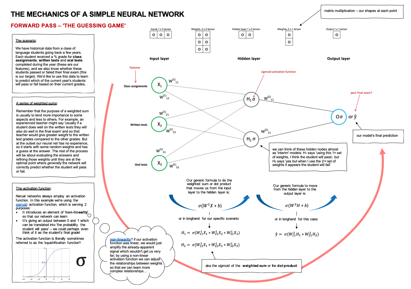
Our first step, in order to move from the input layer to the hidden layer, is therefore to find the dot product of our inputs and our weights (take note of the tensor shapes involved here).
Our second step is to apply an activation function to the result. Activation functions are part of the secret sauce that enables neural networks to train effectively. In our example, we’re using the sigmoid activation function which is serving 2 purposes:
- It introduces an element of ‘non-linearity‘ so that our network can learn. After all, if what we were trying to learn involved a simple linear relationship we could just use linear regression to predict whether students would pass or fail. However, if we’ve established that ‘it’s more complicated than that’ and ‘it depends’, we don’t want to just amplify the linear signals that already exist in our data, we want to learn more complex non-linear relationships that will ultimately lead to a correct prediction on pass or fail. We said earlier that our experienced teacher might intuitively know that if a student does well on the written tests they will usually do well in the final exam. But she might also be aware that as long as the student gets more than 50% on any 2 of the evaluation components they’re likely to pass the final exam, or if they get 80% or more on class assignments they’re likely to pass, and so on. By using a non-linear activation function we can adjust the relationships between weights so that we can learn these more complex relationships…
- The second purpose our activation function serves here is to ensure our output is a number between 0 and 1 which can be translated into ‘the probability the student will pass’ – we could perhaps even think of it as the student’s final grade.
There are several popular activation functions used in neural networks, including tanh, relu, sigmoid.
Having made it to the hidden layer, we can think of those 2 hidden nodes almost as ‘preliminary guesses’ in the guessing game! Node 1 might say ‘I think the student will pass with 80%’, while Node 2 might say ‘I think the student will fail with 30%’. We then repeat the dot product > activation function process to move from our hidden layer to our output layer (and our final answer). If the weights assigned to Node 1 and Node 2 were equivalent then our final guess would be that the student would pass, BUT it is likely that our network will give one node more weight than the other so it’s equally possible that, by giving more weight to the ‘fail’ Node 2, our final guess is that the student will fail.
Measuring error
Now let’s look at the error part of ‘trial and error’. The function that is used to measure the amount of error is called the error function (how memorable!), but as usual there are a multiplicity of other terms which all mean the same thing so you may see any of these:
- Error function
- Cost function
- Loss function
- Objective function
Whatever we call it, it’s the thing that will measure how big the error is, and our goal will then be to reduce the error (aka minimize the error) at each guess as efficiently as possible to arrive at the correct answer.
There are many different functions that can be used to measure error (this article on Medium has a nice summary of some of the most popular ones).
- Regression-type problems will often use the mean squared error function
- Classification-type problems will often use the cross-entropy loss function
Whatever function you use to measure error there are 2 golden rules:
- The function must be differentiable (because we are going to use Calculus to help us reduce the error efficiently).
- The function must be continuous (not yes or no, but rather a measurement of how wrong or right) – and this makes sense, right? If the teacher just gives feedback ‘you’re wrong’ you don’t know whether you are badly wrong or a little bit wrong, nor do you know in which direction to guess next).
In our scenario we will use the binary cross-entropy error function which is commonly used in ‘yes-no’, ‘pass-fail’, ‘win-lose’ type of scenarios.
Back propagation – the blame game
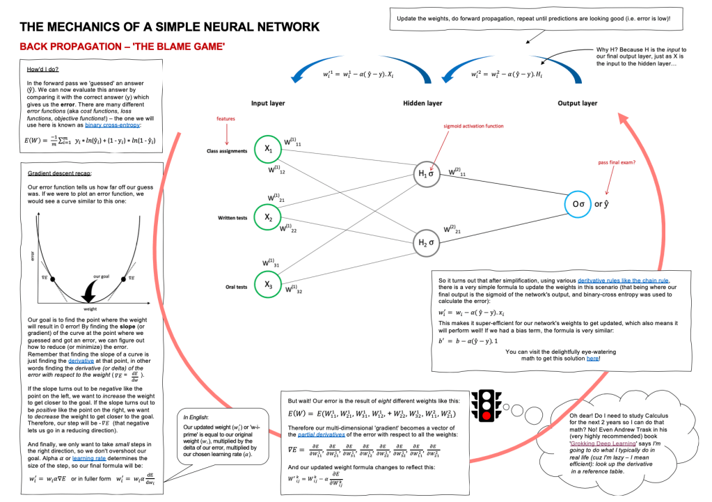
We can think of gradient descent as the method we use for finding a more optimal route from the initial random guess to the eventual correct answer. Let’s come back for a moment to our student who was trying to learn that 1 + 5 = 6 by guessing. His first guess was 19. If his second guess, after receiving feedback that 19 was too high, was to try -24, you can imagine that he might spend quite a lot of time guessing: too high, too low, too high again, etc. Whereas if he cautiously amends his guess each time, maybe choosing 16, then 12, then 8, then 4, and finally 6, he’ll get there a lot faster. Controlling this cautious amendment of guesses is what gradient descent is all about.
Our goal is to find the point where the weights will result in 0 error (or as near as we can get to 0 error – this is not Utopia after all). By finding the slope (or gradient) of the curve at the point where we guessed and got an error, we can figure out how to reduce (or minimize) the error. Remember that finding the slope of a curve is just finding the derivative at that point, in other words finding the derivative (or delta) of the error with respect to the weight.
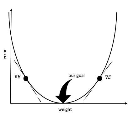
If the slope turns out to be negative like the point on the left, we want to increase the weight to get closer to the goal. If the slope turns out to be positive like the point on the right, we want to decrease the weight to get closer to the goal. And finally, we only want to take small steps in the right direction, so we don’t overshoot our goal. Alpha or the learning rate determines the size of the step we take after learning new information at the end of each round of guessing.
The complexity of doing this in a neural network is that there is not just ONE weight to adjust but many: 100’s or 1000’s or more… and each one must be assigned their share of the blame! Therefore the ‘gradient’ or ‘slope’ becomes a multi-dimensional vector of the partial derivatives of the error with respect to all of the weights. There is some eye-watering math you can do to calculate this manually (Matt Mazur’s step-by-step example showcases exactly how this works if you want the nitty gritty detail), but fortunately in practice, PyTorch or Tensorflow or similar libraries, will take care of this step for you.
Repeat…
This process is repeated as many times as is necessary until the error has been reduced to an acceptably low level, and you are satisfied with your predictions!
